How to Read Spss Results Anova Repeated Measures
In this tutorial, we'll look at how to perform a repeated-measures (or inside-subjects) ANOVA in SPSS, and also at how to translate the result.
A repeated-measures ANOVA design is sometimes used to analyze data from a longitudinal study, where the requirement is to assess the result of the passage of time on a particular variable. For this tutorial, we're going to utilize data from a hypothetical study that looks at whether fear of spiders among arachnophobes increases over fourth dimension if the disorder goes untreated.
Quick Steps
- Click Clarify -> General Linear Model -> Repeated Measures
- Proper noun your Inside-Subject factor, specify the number of levels, then click Add together
- Hit Ascertain, and then drag and drop (left to right) a variable for each of the levels yous specified (taking care to preserve their right order)
- Click Options, and tick the Descriptive statistics and Estimate of effect size boxes, then click Continue
- You're now ready to run the examination. Printing the OK push, and your issue will pop up in the Output Viewer
The Data
This is the data from our "report" every bit it appears in the SPSS Information View.
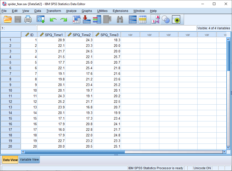
The variable we're interested in here is SPQ which is a measure of the fear of spiders that runs from 0 to 31. The average score for a person with a spider phobia is 23, which compares to a score of slightly under 3 for a non-phobic.
SPQ is the dependent variable. The contained variable – or, to adopt the terminology of ANOVA, the within-subjects factor – is time, and it has three levels: SPQ_Time1 is the time of the first SPQ assessment; SPQ_Time2 is one year later; and SPQ_Time3 two years later.
The null hypothesis is that the hateful SPQ score is the same for all levels of the inside-subjects gene. This is what nosotros'll exam with a i-way repeated-measures ANOVA.
Repeated-Measures ANOVA
To offset, click Analyze -> Full general Linear Model -> Repeated Measures. This will bring up the Repeated Measures Define Gene(s) dialog box.
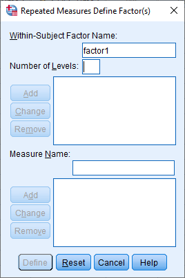
As we noted above, our inside-subjects gene is time, so type "fourth dimension" in the Within-Subject area Factor Name box. And we have 3 levels, so input 3 into Number of Levels. So click Add.
The dialog box should now expect similar this.
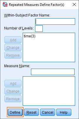
Okay, it'south now time to gear up up the within-subjects variables (at the moment SPSS knows that our inside-subjects factor has iii levels, but it doesn't know which of our variables corresponds to each level). Click on the Define button, which volition bring upwardly the Repeated Measures dialog blox.
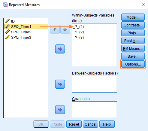
Yous've got to shift your within-subjects variables over to the Within-Subjects Variables box ensuring you maintain the right lodge. You lot tin can drag and driblet, or use the arrow push button in the centre of the box. In our case, it just means moving SPQ_Time1, SPQ_Time2 & SPQ_Time3 into the three slots on the right.
The dialog box should look something like this once you've completed this stage.
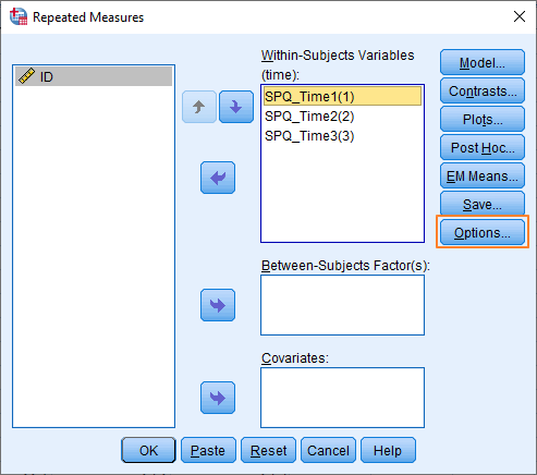
We're now ready to ready some of the options for the repeated-measures ANOVA. Click on the Options button.
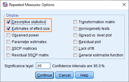
Options
What you lot see here depends on the version of SPSS yous're using. The most recent version of SPSS (26) has an options dialog box that looks like this.
Previous versions include an choice for specifying estimated marginal means. It looks like this.
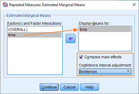
We're going to assume that you're using a previous version of SPSS, and you're seeing the estimated marginal means option. If you're not, and then you need to click on the EM Ways push (in the Repeated Measures dialog box) later on you've finished with the Options dialog box, and set upwards the estimated marginal ways there.
It'south not too difficult to get the options sorted out. Y'all want to display descriptive statistics and estimates of effect size, then tick these options in the Display section (every bit to a higher place). So in the Estimated Marginal Ways section (or dialog box if you're using the current version of SPSS), move "time" over to the Brandish Means for box, and then tick Compare chief effects, and choose Bonferroni equally the Confidence interval adjustment option.
Hitting the Continue button(s) once you lot've got this set up.
That's it, you're ready to run the examination. You should be looking at the original Repeated Measures dialog box. All you've got to do is hit OK, and you'll encounter the result pop up in the Output Viewer.
The Effect
SPSS produces a lot of output for the 1-way repeated-measures ANOVA test. For the purposes of this tutorial, we're going to concentrate on a adequately simple estimation of all this output. (In future tutorials, we'll look at some of the more than complex options bachelor to you, including multivariate tests and polynomial contrasts).
Descriptive Statistics
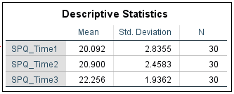
The descriptive statistics that SPSS outputs are easy enough to understand. The comparison between means (meet above) gives us an idea of the management of any possible effect. In our example, it seems as if fear of spiders increases over time, with the greatest increment (20.90 to 22.26 on the SPQ scale) occurring betwixt year 1 (SPQ_Time2) and year 2 (SPQ_Time3). Of course, we won't know whether these differences in the means reach significance until we look at the upshot of the ANOVA test.
Assumption of Sphericity
A requirement that must be met before you can trust the p-value generated past the standard repeated-measures ANOVA is the homogeneity-of-variance-of-differences (or sphericity) assumption. For our purposes, it doesn't affair too much what this means, we just need to know how to figure out whether the requirement has been satisfied.
SPSS tests this supposition by running Mauchly'southward examination of sphericity.
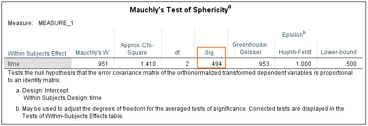
What we're looking for here is a p-value that's greater than .05. Our p-value is .494, which ways nosotros meet the supposition of sphericity.
You've got to be careful here. This assumption is frequently violated. If information technology is, in guild to summate a reliable value forp, you'll need to adapt the degrees of liberty of F in line with the extent to which the assumption is violated. Happily SPSS does this work for you. All you lot've got to do is choose an alternative univariate test. Let'southward look at this now.
Tests of Within-Subjects Effects
This is where nosotros read off the result of the repeated-measures ANOVA exam.
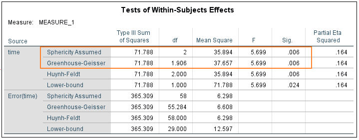
Every bit we accept only discussed, our data meets the assumption of sphericity, which ways we can read our outcome straight from the summit row (Sphericity Causeless). The value of F is 5.699, which reaches significance with a p-value of .006 (which is less than the .05 alpha level). This ways in that location is a statistically meaning difference between the means of the unlike levels of the within-subjects variable (time).
If our information had not met the assumption of sphericity, nosotros would need to employ one of the alternative univariate tests. You lot'll observe that these produce the same value for F, just that there is some variation in the reported degrees of freedom. In our case, there is not enough deviation to modify the p-value – Greenhouse-Geisser and Huynh-Feldt, both produce pregnant results (p = .006).
Pairwise Comparisons
Although nosotros know that the differences betwixt the means of our three within-subjects levels are large enough to reach significance, we don't withal know between which of the various pairs of means the difference is pregnant. This is where pairwise comparisons come into play.
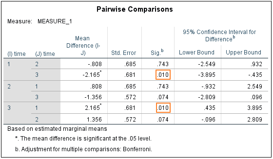
This table features threeunique comparisons between the means for SPQ_Time1, SPQ_Time2 and SPQ_Time3. Simply one of the differences reaches significance, and that'due south the difference between the means for SPQ_Time1 and SPQ_Time iii (see in a higher place). It is worth noting that SPSS is using an adapted p-value here in order to control for multiple comparisons, and that the program lets you know if a mean difference has reached significance by attaching an asterisk to the value in cavalcade 3.
Report the Effect
When reporting the consequence information technology's normal to reference both the ANOVA test and any postal service hoc assay that has been done.
Thus, given our case, you could write something similar:
A repeated-measures ANOVA adamant that mean SPQ scores differed significantly across three time points (F(2, 58) = 5.699, p = .006). A post hoc pairwise comparing using the Bonferroni correction showed an increased SPQ score between the initial cess and follow-up assessment one twelvemonth later (twenty.1 vs 20.9, respectively), but this was non statistically significant (p = .743). However, the increase in SPQ score did accomplish significance when comparing the initial assessment to a second follow-up assessment taken two years after the original cess (twenty.1 vs 22.26, p = .010). Therefore, we tin conclude that the results for the ANOVA indicate a significant time consequence for untreated fear of spiders equally measured on the SPQ scale.
***************
Okay, that'southward all for this tutorial. You should now exist able to run a repeated-measures ANOVA, exam the supposition of sphericity, make utilise of a pairwise comparison, and study the event. In future tutorials, we'll look at some of the more sophisticated options available for this exam. Simply this tutorial should provide enough information for you to run a basic repeated-measures ANOVA test.
Source: https://ezspss.com/repeated-measures-anova-in-spss-including-interpretation/
0 Response to "How to Read Spss Results Anova Repeated Measures"
Post a Comment